
Gradient boosting builds a strong prediction model by adding many small decision trees one after another, where each new tree is trained to fix the mistakes the earlier trees still make. Libraries and papers call the result a GBM, short for gradient boosting machine. It is the method behind many winning entries in competitions on tabular data, and it is simpler than its reputation.
In this tutorial we build gradient boosting from scratch in about 15 lines of Python, check that it gives the same predictions as scikit-learn’s implementation, and then use scikit-learn to tune it, test it for overfitting and compare it with other models. All numbers below come from running the code on the classic car fuel economy data (392 cars, seaborn’s mpg dataset).
How gradient boosting works in plain words
Imagine predicting a car’s fuel economy. You start with the dumbest possible guess: the average mpg of every car. That guess is wrong for most cars, so you measure the errors (the residuals). Then you train a small decision tree to predict those errors, and add a fraction of its output to your guess. The new guess is a little better. You measure the remaining errors, train another small tree on them, and repeat.
Each tree is weak on its own, because it is only two or three levels deep. Added together, a hundred of them make a flexible model. Two settings control the process: the number of trees and the learning rate, the fraction of each tree’s output that you add. A small learning rate takes smaller steps and needs more trees.
This differs from a random forest, which trains many deep trees independently and averages them. Boosting trains small trees in sequence, each one depending on the last. If you know AdaBoost, it is a close relative that re-weights the examples instead of fitting residuals; see our AdaBoost guide.
Build gradient boosting from scratch
You need Python with numpy, seaborn and scikit-learn (we used scikit-learn 1.9.1, pandas 3.0.5 and seaborn 0.13.2). We predict mpg from horsepower alone first, because one feature lets us draw what the model learns. Six cars have no horsepower value, so dropna() leaves 392.
import numpy as np
import seaborn as sns
from sklearn.ensemble import GradientBoostingRegressor
from sklearn.tree import DecisionTreeRegressor

# --- Step 1: load the data
cars = sns.load_dataset("mpg").dropna()          # 392 cars
X = cars[["horsepower"]].to_numpy()
y = cars["mpg"].to_numpy()


# --- Step 2: gradient boosting in 15 lines
class MyGBM:
    def __init__(self, n_estimators=100, learning_rate=0.1, max_depth=2):
        self.n, self.lr, self.depth = n_estimators, learning_rate, max_depth

    def fit(self, X, y):
        self.base = y.mean()                      # start from the average
        self.trees = []
        pred = np.full(len(y), self.base)
        for _ in range(self.n):
            residual = y - pred                   # what we still get wrong
            tree = DecisionTreeRegressor(max_depth=self.depth, random_state=0)
            tree.fit(X, residual)                 # a small tree learns the errors
            pred = pred + self.lr * tree.predict(X)
            self.trees.append(tree)
        return self

    def predict(self, X, upto=None):
        pred = np.full(len(X), self.base)
        for tree in self.trees[:upto]:
            pred = pred + self.lr * tree.predict(X)
        return pred
The class does exactly what we described. It stores the average as its starting guess, then loops: compute the residual, fit a depth-2 tree to it, and add learning_rate times the tree’s prediction. Prediction replays the same steps. The upto argument lets us stop after the first k trees, which is useful for watching the model grow.
# --- Step 3: watch the error fall as trees are added
model = MyGBM(n_estimators=100, learning_rate=0.1, max_depth=2).fit(X, y)
for k in (0, 1, 5, 20, 100):
    mse = ((y - model.predict(X, upto=k)) ** 2).mean()
    print(f"{k:>3} trees: training MSE {mse:.2f}")

# --- Step 4: compare with scikit-learn
ref = GradientBoostingRegressor(n_estimators=100, learning_rate=0.1,
                                max_depth=2, random_state=0).fit(X, y)
print("largest difference:", np.abs(model.predict(X) - ref.predict(X)).max())
Running it prints the training error after 0, 1, 5, 20 and 100 trees:
| Trees | Training MSE |
|---|---|
| 0 (just the average) | 60.76 |
| 1 | 52.73 |
| 5 | 32.98 |
| 20 | 17.35 |
| 100 | 13.69 |
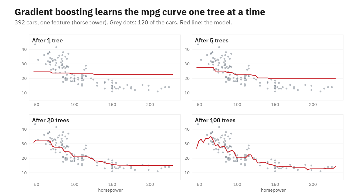
With zero trees the error equals the variance of mpg, 60.76, because we predict the average for every car. One tree removes some of it, and by 100 trees the error is about a fifth of where it started. The figure shows what the model looks like at each stage.
Check it against scikit-learn
The last lines of the script train scikit-learn’s GradientBoostingRegressor with the same settings and compare predictions. The largest difference between our 15 lines and the library is 0.0. The two models make identical predictions on every car, so what you just wrote is real gradient boosting. The library adds speed, other loss functions and many options on top.
Why is it called “gradient” boosting?
We fitted each tree to the residual, y - prediction. For squared error, the residual is exactly the negative gradient of the loss with respect to the current prediction, which is where the name comes from. This matters because the gradient view generalises: for other losses the tree is fitted to a different quantity. With absolute error it is the sign of the residual, and with log loss for classification it is the true label minus the predicted probability. The loop stays the same, and only the thing the trees learn changes. In scikit-learn you pick it with the loss parameter.
Tune the learning rate and the number of trees
Now we use all six numeric features and judge models properly with 5-fold cross-validation, which scores every car on a model that never saw it. The metric is mean absolute error (MAE) in mpg, so lower is better. Here is the grid of learning rates and tree counts, with trees of depth 3:
import numpy as np, seaborn as sns
from sklearn.ensemble import GradientBoostingRegressor, RandomForestRegressor, HistGradientBoostingRegressor
from sklearn.dummy import DummyRegressor
from sklearn.linear_model import LinearRegression
from sklearn.model_selection import KFold, cross_val_score, train_test_split
from sklearn.metrics import mean_absolute_error
from sklearn.inspection import permutation_importance

# --- Step 5: tune the learning rate and the number of trees
cars = sns.load_dataset("mpg").dropna()
features = ["cylinders", "displacement", "horsepower", "weight", "acceleration", "model_year"]
X, y = cars[features], cars["mpg"]
cv = KFold(5, shuffle=True, random_state=0)

def cv_mae(model):
    return -cross_val_score(model, X, y, cv=cv, scoring="neg_mean_absolute_error").mean()

for lr in (0.01, 0.1, 0.5, 1.0):
    scores = [cv_mae(GradientBoostingRegressor(n_estimators=n, learning_rate=lr, max_depth=3, random_state=0))
              for n in (50, 200, 500)]
print(lr, [round(float(s), 2) for s in scores])| Learning rate | 50 trees | 200 trees | 500 trees |
|---|---|---|---|
| 0.01 | 4.42 | 2.29 | 1.99 |
| 0.1 | 1.98 | 2.00 | 2.05 |
| 0.5 | 2.05 | 2.08 | 2.08 |
| 1.0 | 2.57 | 2.60 | 2.60 |
Predicting the average for every car gives an MAE of 6.57, so even the weakest cell here learns something. Three patterns show up:
- A small learning rate needs many trees. At 0.01, 50 trees are not enough (4.42), but 500 reach 1.99.
- A medium rate gets there fast. At 0.1, 50 trees already give 1.98, and more trees slowly make the score worse (2.05 at 500).
- A learning rate of 1.0 is too aggressive. Every tree is added in full, the model chases noise, and the error stays at 2.57 to 2.60.
The best cells (0.01 with 500 trees and 0.1 with 50) differ by 0.01 mpg, which is nothing. The practical rule: start at 0.1, and only drop to 0.01 or lower if you can afford many more trees.
Watch for overfitting
Boosting keeps fitting the training data as you add trees, so you should compare the training error with the error on cars the model has not seen. Here we hold out 20% of the cars (79 of them) and score the model after every tree:
# --- Step 6: train error versus test error
X_train, X_test, y_train, y_test = train_test_split(X, y, test_size=0.2, random_state=0)
gbm = GradientBoostingRegressor(n_estimators=500, learning_rate=0.1, max_depth=3, random_state=0).fit(X_train, y_train)
train_mae = [mean_absolute_error(y_train, p) for p in gbm.staged_predict(X_train)]
test_mae = [mean_absolute_error(y_test, p) for p in gbm.staged_predict(X_test)]
for k in (50, 100, 500):
print(f"{k:>3} trees: train MAE {train_mae[k-1]:.2f}, test MAE {test_mae[k-1]:.2f}")| Trees | Train MAE | Test MAE |
|---|---|---|
| 50 | 1.33 | 1.76 |
| 100 | 1.06 | 1.79 |
| 500 | 0.27 | 1.80 |
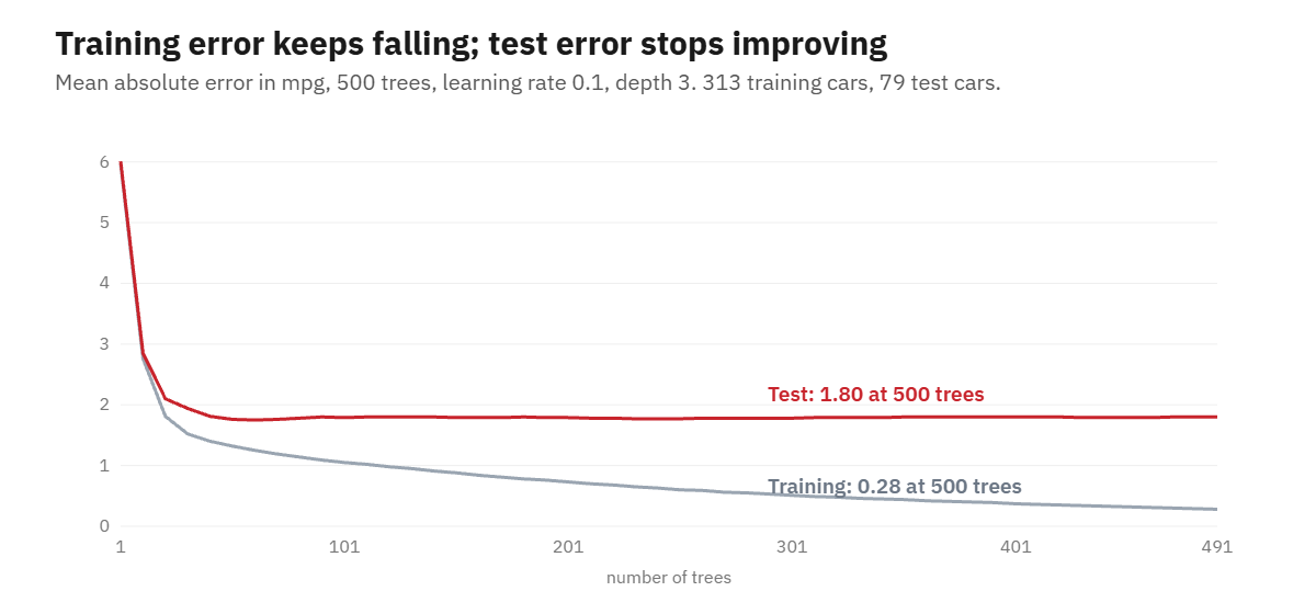
Training error falls from 1.33 to 0.27 while test error does not move. The model memorises the 313 training cars better and better without learning anything new about cars in general. On this data the test error stays flat instead of climbing, because the trees are shallow and the learning rate is small, but the extra 450 trees are pure cost. With only 79 test cars, differences of 0.05 mpg are noise, so do not read much into which tree count is “best”.
Your tools against overfitting are the ones from the grid above: fewer trees, a smaller learning rate, shallower trees (max_depth) and subsample below 1.0, which trains each tree on a random part of the data. scikit-learn can also stop for you: set n_iter_no_change and it halts when a validation score stops improving.
Compare it with other models
# --- Step 7: compare with other models (5-fold cross-validation)
models = {"average": DummyRegressor(), "linear regression": LinearRegression(),
          "random forest": RandomForestRegressor(300, random_state=0, n_jobs=2),
          "gradient boosting": GradientBoostingRegressor(random_state=0),
          "HistGradientBoosting": HistGradientBoostingRegressor(random_state=0)}
for name, m in models.items():
print(f"{name:<22} {cv_mae(m):.2f}")| Model | Cross-validated MAE (mpg) |
|---|---|
| Average of all cars | 6.57 |
| Linear regression | 2.68 |
| Random forest | 1.92 |
| Gradient boosting (defaults) | 1.98 |
| HistGradientBoosting | 1.96 |
Gradient boosting cuts the error of linear regression by about 26% (2.68 to 1.98), because fuel economy does not fall in a straight line with weight and horsepower. It does not beat the random forest here: 1.98 against 1.92 is well inside the noise, since the fold-to-fold spread is about 0.14. Boosting is not automatically better, and on a small, clean dataset like this one a forest is just as good. Its advantage tends to show on larger data, with careful tuning.
See which features matter
# --- Step 8: which features matter
imp = permutation_importance(gbm, X_test, y_test, scoring="neg_mean_absolute_error", n_repeats=20, random_state=0)
for i in np.argsort(-imp.importances_mean):
print(f"{features[i]:<13} {imp.importances_mean[i]:.2f}")| Feature | Increase in test MAE when shuffled |
|---|---|
| weight | 2.79 |
| model_year | 2.30 |
| horsepower | 1.37 |
| displacement | 0.89 |
| cylinders | 0.43 |
| acceleration | 0.29 |
Permutation importance shuffles one column and measures how much the error grows. Weight and model year matter most: heavier cars drive fewer miles per gallon, and newer cars are more efficient than older ones with the same weight. Shuffling acceleration barely changes the result. Cylinders and displacement carry information that weight and horsepower already hold, so each looks less important than it would alone.
Which library should you use?
For small data like this, scikit-learn’s GradientBoostingRegressor is fine. For data beyond a few tens of thousands of rows, use HistGradientBoostingRegressor (also in scikit-learn), which is much faster and handles missing values natively, or one of the dedicated libraries. We benchmarked XGBoost, LightGBM and CatBoost for speed and accuracy in XGBoost vs LightGBM vs CatBoost. If you want the full scikit-learn workflow around a model, see our scikit-learn tutorial.
When to use gradient boosting, and when not to
- Use it for tabular data (rows and columns) with a mix of numeric features, where you want high accuracy without much preprocessing.
- Avoid it for images, audio and raw text, where neural networks such as CNNs do better.
- Be careful when you need predictions outside the range of your training data. Trees cannot extrapolate: the red line in the figure goes flat at the edge, while a linear model would carry on.
Common problems
- The score gets worse as you add trees. Lower the learning rate or use early stopping.
- Training error is tiny but test error is not. The model is memorising. Reduce
max_depth, addsubsample=0.8or use fewer trees. - Results change from run to run. Set
random_state. Boosting itself is deterministic, but tree splits can tie, andsubsampleadds randomness. - You tuned on the test set. Choose settings with cross-validation or a validation split, and touch the test set once at the end.
Frequently asked questions
What is gradient boosting in simple terms?
It is a method that builds a model from many small decision trees, adding them one at a time. Each tree learns to correct the errors left by the trees before it.
What does GBM stand for?
GBM stands for gradient boosting machine. The term can mean the general method or a specific implementation, such as scikit-learn’s GradientBoostingRegressor.
What is the difference between boosting and bagging?
Bagging, as in a random forest, trains models independently on random samples and averages them. Boosting trains models in sequence, and each model focuses on the errors of the previous ones.
How many trees do I need?
It depends on the learning rate. With a rate of 0.1, 50 to 200 trees is a good place to start. Choose the number with cross-validation or early stopping, not by looking at training error.
Can gradient boosting do classification?
Yes. The same loop works with a classification loss, and each tree then learns the gap between the true label and the predicted probability. In scikit-learn use GradientBoostingClassifier.
