
TensorFlow is Google’s open-source library for building and training neural networks. Its high-level API, Keras, lets you define a network in a few lines, train it with one call to fit, and save it for use in an app.
This tutorial starts with the two ideas everything else is built on, tensors and automatic gradients, then builds a real neural network that predicts the price of 54,000 diamonds. Along the way it compares the network with simpler models, because a neural network isn’t always the best choice. Every output shown is what the code printed when we ran it, using TensorFlow 2.21 and Keras 3.
Install TensorFlow
pip install tensorflow scikit-learn pandas seaborn matplotlibTensorFlow runs on Windows, macOS and Linux with a recent 64-bit version of Python. Everything in this guide runs on an ordinary laptop CPU; you don’t need a GPU. If the install fails, check that your Python version is one TensorFlow currently supports, and install into a fresh virtual environment.
Tensors: TensorFlow’s arrays
A tensor is a multi-dimensional array, like a NumPy array, that TensorFlow can run on a CPU or GPU and track for gradients. Every input, weight and output in a neural network is a tensor.
import tensorflow as tf

a = tf.constant([[1.0, 2.0], [3.0, 4.0]])
b = tf.constant([[1.0], [0.5]])

print(a.shape, a.dtype)
print(tf.matmul(a, b))
print((a * 10).numpy())
Output:
(2, 2) <dtype: 'float32'>
tf.Tensor(
[[2.]
 [5.]], shape=(2, 1), dtype=float32)
[[10. 20.]
 [30. 40.]]
A tensor has a shape and a data type. tf.matmul multiplies matrices, ordinary operators work element by element, and .numpy() converts a tensor back to a NumPy array.
Automatic differentiation with GradientTape
Training a neural network means repeatedly nudging its weights in the direction that reduces the error. To know which direction that is, you need the gradient: how much the error changes when each weight changes. TensorFlow calculates gradients for you. Record a calculation inside a tf.GradientTape and ask for the derivative:
x = tf.Variable(2.0)

with tf.GradientTape() as tape:
    y = x ** 2 + 3 * x

print(tape.gradient(y, x).numpy())   # dy/dx = 2x + 3 = 7 at x = 2
Output:
7.0The derivative of x² + 3x is 2x + 3, which is 7 at x = 2. TensorFlow worked that out without being told the formula.
Train a model by hand
That’s enough to train a model. Generate 200 points along the line y = 3x + 2 with some noise, start with a guess of 0 for both the slope and the intercept, and repeat: predict, measure the error, compute the gradients and take a small step downhill.
tf.random.set_seed(0)
x_data = tf.random.uniform((200, 1), -1, 1)
y_data = 3 * x_data + 2 + tf.random.normal((200, 1), stddev=0.1)

w = tf.Variable(0.0)
b = tf.Variable(0.0)
learning_rate = 0.1

for step in range(1, 201):
    with tf.GradientTape() as tape:
        pred = w * x_data + b
        loss = tf.reduce_mean((pred - y_data) ** 2)
    dw, db = tape.gradient(loss, [w, b])
    w.assign_sub(learning_rate * dw)
    b.assign_sub(learning_rate * db)
    if step in (1, 10, 50, 200):
        print(f"step {step:3}: loss {loss.numpy():.4f}  w {w.numpy():.3f}  b {b.numpy():.3f}")
Output:
step   1: loss 6.7797  w 0.190  b 0.389
step  10: loss 0.9865  w 1.463  b 1.754
step  50: loss 0.0144  w 2.910  b 2.000
step 200: loss 0.0104  w 3.013  b 2.003
After 200 steps the model has found a slope of 3.013 and an intercept of 2.003, almost exactly the true values. This loop of predict, measure, compute gradients and update is gradient descent, and it’s what every neural network does during training. Keras runs the same loop for you, with millions of weights instead of two.
Build a neural network with Keras
Step 1: Load the data
The diamonds dataset, included with seaborn, has the price and characteristics of 53,940 diamonds: weight in carats, quality of cut, color, clarity and physical dimensions.
import numpy as np
import pandas as pd
import seaborn as sns

diamonds = sns.load_dataset("diamonds")
print(diamonds.shape)
print(diamonds.head(3))
print(diamonds["price"].describe()[["min", "50%", "max"]])
Output:
(53940, 10)
   carat      cut color clarity  depth  table  price     x     y     z
0   0.23    Ideal     E     SI2   61.5   55.0    326  3.95  3.98  2.43
1   0.21  Premium     E     SI1   59.8   61.0    326  3.89  3.84  2.31
2   0.23     Good     E     VS1   56.9   65.0    327  4.05  4.07  2.31
min      326.0
50%     2401.0
max    18823.0
Name: price, dtype: float64
Prices range from $326 to $18,823, with a median of $2,401. Because prices are so skewed, the model will predict the logarithm of the price. That way an error of 10% counts the same for a cheap diamond as for an expensive one.
Step 2: Prepare the features
Neural networks need numbers, so turn the text columns (cut, color and clarity) into 0/1 columns with get_dummies, then hold back 20% of the diamonds for the final test.
from sklearn.model_selection import train_test_split

X = pd.get_dummies(diamonds.drop(columns="price"), dtype="float32")
y = np.log(diamonds["price"]).astype("float32")      # predict log price

X_train, X_test, y_train, y_test = train_test_split(X, y, test_size=0.2, random_state=0)
print(X.shape[1], "features")
print(len(X_train), "training rows,", len(X_test), "test rows")
Output:
26 features
43152 training rows, 10788 test rows
Step 3: Set a baseline
Before building a neural network, find out what a simple model can do. If the network can’t beat it, the network isn’t worth the extra complexity. The helper converts predictions back from log price to dollars and reports the mean absolute error (MAE): how far off the predicted price is, on average.
from sklearn.linear_model import LinearRegression
from sklearn.metrics import mean_absolute_error

def dollar_mae(log_true, log_pred):
    return mean_absolute_error(np.exp(log_true), np.exp(log_pred))

lin = LinearRegression().fit(X_train, y_train)
print(f"linear regression MAE: ${dollar_mae(y_test, lin.predict(X_test)):,.0f}")
Output:
linear regression MAE: $472Linear regression is off by $472 per diamond on average. That’s the number to beat.
Step 4: Define the network
import keras
from keras import layers

keras.utils.set_random_seed(0)

normalizer = layers.Normalization()
normalizer.adapt(X_train.to_numpy())

model = keras.Sequential([
    keras.Input(shape=(X.shape[1],)),
    normalizer,
    layers.Dense(64, activation="relu"),
    layers.Dense(64, activation="relu"),
    layers.Dense(1),
])
model.compile(optimizer=keras.optimizers.Adam(learning_rate=0.001), loss="mse", metrics=["mae"])
print(model.count_params(), "parameters")
Output:
6006 parametersEach part of the model has a job:
- Normalization rescales every feature to a mean of 0 and a standard deviation of 1.
adaptlearns those statistics from the training data only. Without it, columns with large values, such as table (around 57), would swamp the 0/1 columns and training would be slow and unstable. - Two Dense layers of 64 units with the ReLU activation do the learning. Each unit computes a weighted sum of its inputs and passes it through ReLU, which outputs the value if it’s positive and 0 otherwise. Stacking them lets the network learn curved, interacting relationships, such as price rising faster than carat weight.
- A final Dense layer with one unit and no activation outputs the predicted log price.
- The loss is mean squared error, the standard choice for predicting a number, and Adam is the optimizer, a version of gradient descent that adapts its step size for each weight.
The network has about 6,000 weights to learn.
Step 5: Train it
Keep 20% of the training rows aside for validation and use early stopping, which halts training when the validation loss hasn’t improved for 10 epochs and restores the best weights.
early = keras.callbacks.EarlyStopping(monitor="val_loss", patience=10, restore_best_weights=True)

history = model.fit(X_train, y_train, validation_split=0.2, epochs=200,
                    batch_size=256, callbacks=[early], verbose=0)

print("epochs run:", len(history.history["loss"]))
print("best validation loss:", round(min(history.history["val_loss"]), 4))
Output:
epochs run: 200
best validation loss: 0.0124
import matplotlib.pyplot as plt
fig, ax = plt.subplots(figsize=(7, 4))
ax.plot(history.history["loss"], label="training loss")
ax.plot(history.history["val_loss"], label="validation loss")
ax.set_xlabel("Epoch")
ax.set_ylabel("Mean squared error (log price)")
ax.set_ylim(0, 0.1)
ax.legend()
plt.show()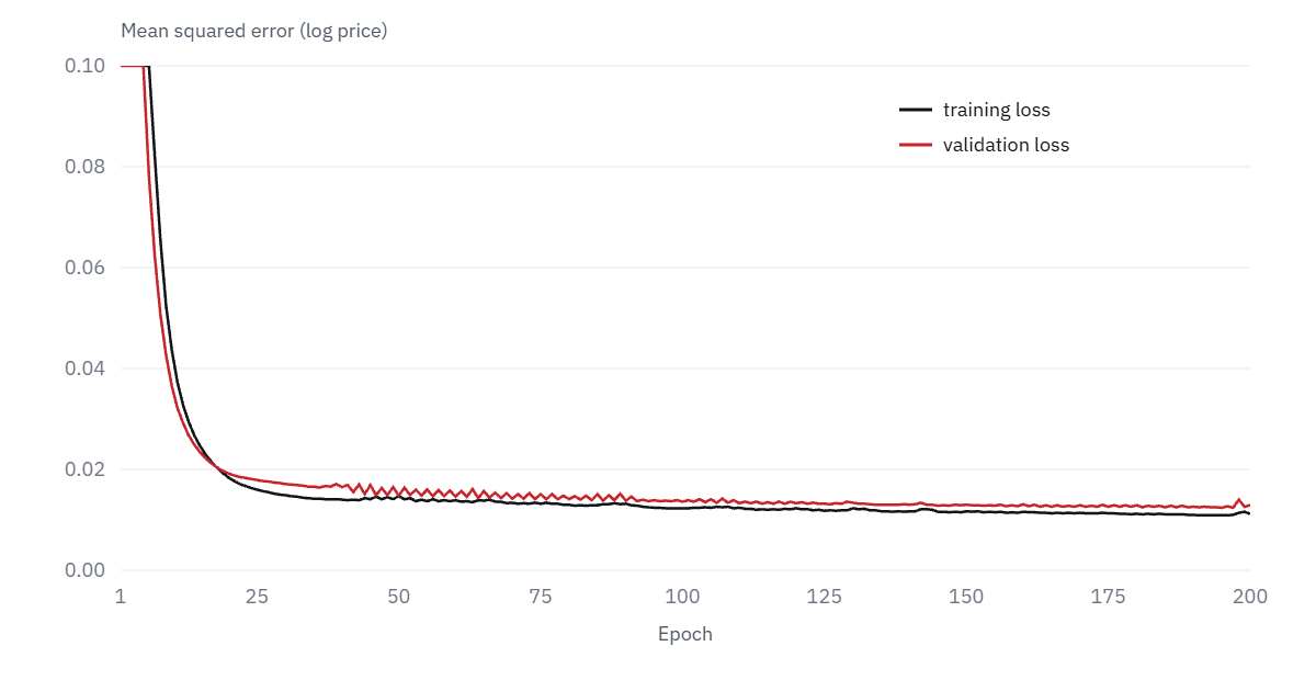
Most of the improvement happens in the first 20 epochs. After that the loss keeps creeping down slowly: the validation loss is 0.037 after 10 epochs, 0.015 after 50 and 0.012 at its best, near the end. Training ran all 200 epochs because the validation loss never stalled for 10 epochs in a row. Training and validation loss stay close together, so the model isn’t overfitting.
Step 6: Evaluate on the test set
nn_pred = model.predict(X_test, verbose=0).ravel()
print(f"neural network MAE: ${dollar_mae(y_test, nn_pred):,.0f}")
Output:
neural network MAE: $328The neural network is off by $328 on average, 30% better than linear regression. But is a neural network the best tool for this job? Try gradient boosting, the usual strong model for tables of data:
from sklearn.ensemble import HistGradientBoostingRegressor

gbm = HistGradientBoostingRegressor(random_state=0).fit(X_train, y_train)
print(f"gradient boosting MAE: ${dollar_mae(y_test, gbm.predict(X_test)):,.0f}")
Output:
gradient boosting MAE: $281| Model | Average error (MAE) | Training time on a 2-core CPU |
|---|---|---|
| Linear regression | $472 | Under a second |
| Neural network (TensorFlow) | $328 | About a minute |
| Gradient boosting (scikit-learn) | $281 | About a second |
Gradient boosting wins, with default settings and in about a second of training. That’s typical: on tabular data, models like XGBoost, LightGBM and CatBoost usually match or beat neural networks. Neural networks pull ahead on images, audio and text, where they learn the features themselves. See our guide to convolutional neural networks for an image example.
Step 7: Make a prediction
New data must go through the same preparation as the training data: the same dummy columns in the same order. reindex adds any columns the new row is missing.
new = pd.DataFrame([{"carat": 1.0, "cut": "Ideal", "color": "G", "clarity": "VS1",
                     "depth": 61.8, "table": 56.0, "x": 6.4, "y": 6.4, "z": 3.95}])
new_X = pd.get_dummies(new, dtype="float32").reindex(columns=X.columns, fill_value=0)

print(f"predicted price: ${np.exp(model.predict(new_X, verbose=0)[0, 0]):,.0f}")
Output:
predicted price: $6,623Remember to convert back from log price with np.exp.
Step 8: Save and reload the model
model.save("diamond_price.keras")
reloaded = keras.models.load_model("diamond_price.keras")
print(f"reloaded model MAE: ${dollar_mae(y_test, reloaded.predict(X_test, verbose=0).ravel()):,.0f}")
Output:
reloaded model MAE: $328The .keras file stores the architecture, the trained weights and the Normalization layer’s statistics, so the reloaded model gives identical predictions. To serve it from a web app, see how to deploy a machine learning model with Flask.
How to improve a TensorFlow model
- Tune the learning rate first. It matters more than any other setting. Try values such as 0.003, 0.001 and 0.0003.
- Change the size of the network. More or wider layers can learn more complex patterns but overfit more easily. Watch the gap between training and validation loss.
- Add regularization if it overfits.
layers.Dropout(0.2)between Dense layers, or an L2 penalty on the weights, both help. - Use embeddings for categories with many values.
layers.Embeddinglearns a compact representation instead of hundreds of 0/1 columns. - Track experiments with TensorBoard. Add
keras.callbacks.TensorBoard(log_dir="logs")to the callbacks and runtensorboard --logdir logsto compare runs side by side.
TensorFlow vs PyTorch vs scikit-learn
| TensorFlow / Keras | PyTorch | scikit-learn | |
|---|---|---|---|
| Best for | Neural networks, production deployment | Neural networks, research | Classical machine learning on tables |
| Ease of starting | Easy with Keras | Moderate | Easiest |
| Deployment options | TF Serving, TensorFlow Lite for mobile, TensorFlow.js for browsers | TorchServe, ONNX export | Pickle or joblib files, ONNX |
| GPU support | Yes | Yes | No |
Keras 3 can also run on top of PyTorch or JAX instead of TensorFlow, so the model code in this guide carries over if you switch.
Common mistakes
- Skipping normalization. Unscaled inputs make training slow or unstable. Use a Normalization layer, adapted on training data only.
- Not comparing with a simple baseline. Here, linear regression gave context and gradient boosting beat the network. Always check.
- Evaluating on data used for tuning. Keep a test set aside and only use it at the end.
- Forgetting to undo a target transformation. This model predicts log price; without
np.expthe predictions are meaningless. - Preparing new data differently. Missing or reordered dummy columns silently produce wrong predictions.
- Expecting identical results everywhere. Even with
set_random_seed, results can differ slightly between machines, CPUs and GPUs.
Keep learning
- Convolutional neural networks explained: TensorFlow on images, where neural networks shine
- Recurrent neural networks: networks for sequences and text
- XGBoost vs LightGBM vs CatBoost: the models to beat on tabular data
- Deploy a machine learning model with Flask
The official TensorFlow tutorials are a good next step once you have built the model above.
FAQ
What is TensorFlow used for?
Building, training and deploying machine learning models, especially neural networks for images, text, audio and time series. Models can run on servers, in browsers with TensorFlow.js and on phones with TensorFlow Lite.
What’s the difference between TensorFlow and Keras?
TensorFlow is the underlying library that handles tensors, gradients and hardware. Keras is the high-level API for defining and training models. You use Keras for almost everything and drop down to TensorFlow, for example GradientTape, when you need more control.
Is TensorFlow good for beginners?
Yes, through Keras. A working network takes a dozen lines, as this guide shows. Understanding tensors and gradient descent first, as in the first sections here, makes everything else easier to follow.
Do I need a GPU for TensorFlow?
Not to learn. The network in this guide trains on an ordinary 2-core CPU in about a minute. GPUs help with large image, audio or language models.
Is TensorFlow better than scikit-learn?
They’re for different jobs. Scikit-learn is simpler and often more accurate on tables of data, as gradient boosting was here. TensorFlow is the better choice for neural networks on images, text and other unstructured data.
