
Matplotlib is the library most Python charts are built on. pandas plotting, seaborn and many other tools draw with it, so once you understand Matplotlib you can control any chart in Python, down to the last tick label.
This guide builds the charts you’ll use most, on two real datasets: monthly airline passengers from 1949 to 1960 and 244 restaurant bills with tips. Each example shows the code and the chart it produced, and explains the choices that make a chart easy to read: what to label, what to remove and which chart to use. Everything was run with Matplotlib 3.11 and pandas 3.0.
Install Matplotlib and make your first chart
pip install matplotlib pandasimport matplotlib.pyplot as plt
years = [2019, 2020, 2021, 2022, 2023, 2024]
users = [120, 180, 260, 410, 530, 720]
fig, ax = plt.subplots()
ax.plot(years, users)
ax.set_title("Monthly active users (thousands)")
plt.show()Three lines do the work. plt.subplots() creates a figure (the whole image) and an axes (one chart inside it, with its own x and y axis). ax.plot() draws on the axes, and plt.show() displays the result. In Jupyter, charts appear automatically at the end of a cell; in a script, plt.show() opens a window.
Two ways to write Matplotlib code
You’ll see two styles online. The pyplot style calls functions on plt directly, such as plt.plot(x, y) and plt.title("..."), and Matplotlib works out which chart you mean. The object-oriented style, used in this guide, creates fig, ax and calls methods on them, such as ax.plot() and ax.set_title(). Both draw the same charts, but the object-oriented style stays clear when a figure has several charts, which is where pyplot code gets confusing. Most method names differ only by set_: plt.xlabel() becomes ax.set_xlabel().
Load the data
Both datasets are small CSV files from the seaborn project’s sample data, loaded straight from GitHub with pandas. We add one column, the tip as a percentage of the bill.
import pandas as pd

URL = "https://raw.githubusercontent.com/mwaskom/seaborn-data/master/"
flights = pd.read_csv(URL + "flights.csv")
tips = pd.read_csv(URL + "tips.csv")
tips["tip_pct"] = tips["tip"] / tips["total_bill"] * 100

print(flights.head(3))
print(tips.head(3))
Output:
   year     month  passengers
0  1949   January         112
1  1949  February         118
2  1949     March         132
   total_bill   tip     sex smoker  day    time  size    tip_pct
0       16.99  1.01  Female     No  Sun  Dinner     2   5.944673
1       10.34  1.66    Male     No  Sun  Dinner     3  16.054159
2       21.01  3.50    Male     No  Sun  Dinner     3  16.658734
Line chart: show change over time
Line charts are for values that follow an order, usually time. This one converts the year and month columns into real dates so Matplotlib spaces them correctly, then adds a vertical line with ax.axvline() and an arrow pointing at the highest month with ax.annotate().
flights["date"] = pd.to_datetime(flights["year"].astype(str) + "-" + flights["month"], format="%Y-%B")
peak = flights.loc[flights["passengers"].idxmax()]

fig, ax = plt.subplots(figsize=(8, 4.5))
ax.plot(flights["date"], flights["passengers"], color="#1f4e79", linewidth=1.8)
ax.axvline(pd.Timestamp("1958-01-01"), color="gray", linestyle="--", linewidth=1)
ax.text(pd.Timestamp("1958-03-01"), 150, "1958 slowdown", color="gray")
ax.annotate(f"Peak: {peak['passengers']} in {peak['date']:%b %Y}",
            xy=(peak["date"], peak["passengers"]), xytext=(pd.Timestamp("1953-06-01"), 580),
            arrowprops=dict(arrowstyle="->", color="black"))
ax.set_title("Monthly airline passengers, 1949 to 1960")
ax.set_ylabel("Passengers (thousands)")
ax.spines[["top", "right"]].set_visible(False)
fig.savefig("line.png", dpi=150, bbox_inches="tight")
plt.show()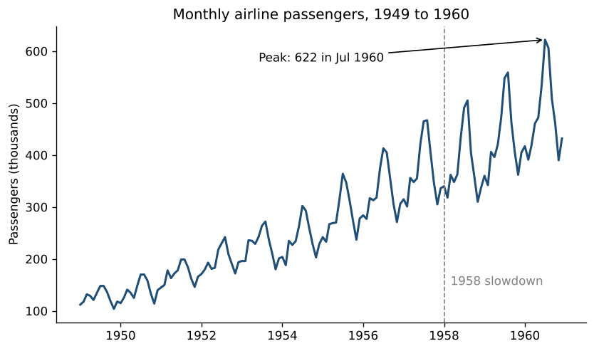
The chart shows two patterns at once: steady growth, and a summer peak every year that gets bigger as the trend rises. The annotation does the reader’s work for them. Instead of making people find the highest point, it tells them what it is. ax.spines[["top", "right"]].set_visible(False) removes the top and right borders, which carry no information; you’ll see it in every example here.
Bar chart: compare categories
Bar charts compare a number across categories. Two choices make them much easier to read: sort the bars so the order means something, and use horizontal bars when labels are long or there are many categories. ax.bar_label() writes each value on its bar, so readers don’t have to estimate from the axis.
by_day = tips.groupby("day")["tip_pct"].mean().sort_values()
print(by_day.round(1))

fig, ax = plt.subplots(figsize=(8, 4))
bars = ax.barh(by_day.index, by_day.values, color="#1f4e79")
ax.bar_label(bars, fmt="%.1f%%", padding=4)
ax.set_title("Average tip by day (% of the bill)")
ax.set_xlabel("Tip (%)")
ax.set_xlim(0, 20)
ax.spines[["top", "right"]].set_visible(False)
fig.savefig("bar.png", dpi=150, bbox_inches="tight")
plt.show()
Output:
day
Sat     15.3
Thur    16.1
Sun     16.7
Fri     17.0
Name: tip_pct, dtype: float64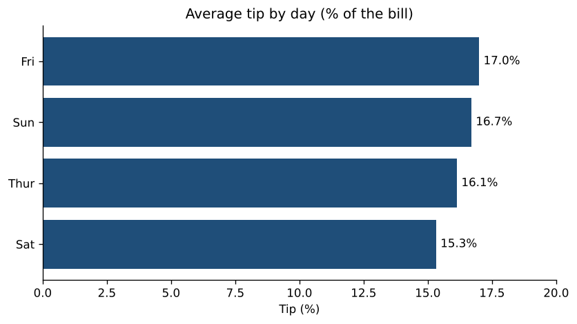
Friday diners tip the most in this data and Saturday diners the least, although the gap is under two percentage points and Friday has only 19 bills, so it could easily be chance. The x-axis starts at zero, which is important for bar charts: because bar length represents the value, a cut-off axis makes small differences look huge. Use ax.bar() instead of ax.barh() for vertical bars.
Histogram: see a distribution
A histogram counts how many values fall into each range (bin), which shows the shape of the data: where most values are, how spread out they are, and whether there are outliers. The vertical line marks the median.
median = tips["tip_pct"].median()

fig, ax = plt.subplots(figsize=(8, 4.5))
ax.hist(tips["tip_pct"], bins=30, range=(0, 75), color="#1f4e79", edgecolor="white")
ax.axvline(median, color="#c8242c", linewidth=2, label=f"Median: {median:.1f}%")
ax.set_title("How much do people tip?")
ax.set_xlabel("Tip (% of the bill)")
ax.set_ylabel("Number of bills")
ax.legend(frameon=False)
ax.spines[["top", "right"]].set_visible(False)
fig.savefig("hist.png", dpi=150, bbox_inches="tight")
plt.show()

print(f"Median {median:.1f}%, highest {tips['tip_pct'].max():.1f}%")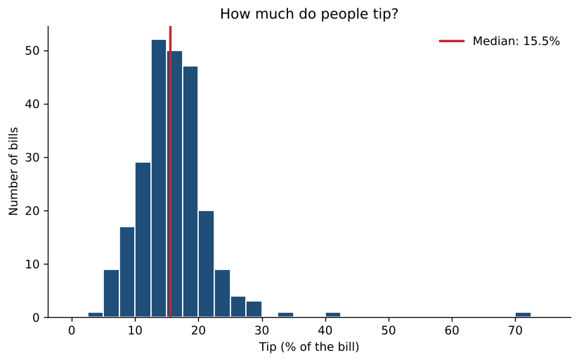
Output:
Median 15.5%, highest 71.0%Most people tip between 10 and 25%, and a few very generous tips stretch the chart to the right. The 71% tip is a $5.15 tip on a $7.25 bill. Try different values for bins: too few hide the shape, too many make it look noisy. 20 to 40 is a good starting range for a few hundred values. Our descriptive statistics calculator draws a histogram and box plot from any list of numbers you paste in.
Scatter plot with a line of best fit
Scatter plots show how two numeric variables relate. Here each dot is a bill, coloured by lunch or dinner, and np.polyfit() fits a straight line through all of them.
import numpy as np

fig, ax = plt.subplots(figsize=(8, 5))
for time, color in [("Lunch", "#e69f00"), ("Dinner", "#1f4e79")]:
    part = tips[tips["time"] == time]
    ax.scatter(part["total_bill"], part["tip"], s=30, alpha=0.7, color=color, label=time)

slope, intercept = np.polyfit(tips["total_bill"], tips["tip"], deg=1)
x = np.linspace(tips["total_bill"].min(), tips["total_bill"].max(), 100)
ax.plot(x, slope * x + intercept, color="black", linewidth=1.5,
        label=f"Best fit: tip = {slope:.3f} × bill + {intercept:.2f}")

ax.set_title("Bigger bills, bigger tips")
ax.set_xlabel("Total bill ($)")
ax.set_ylabel("Tip ($)")
ax.legend(frameon=False)
ax.spines[["top", "right"]].set_visible(False)
fig.savefig("scatter.png", dpi=150, bbox_inches="tight")
plt.show()

print(f"slope {slope:.3f}, intercept {intercept:.2f}")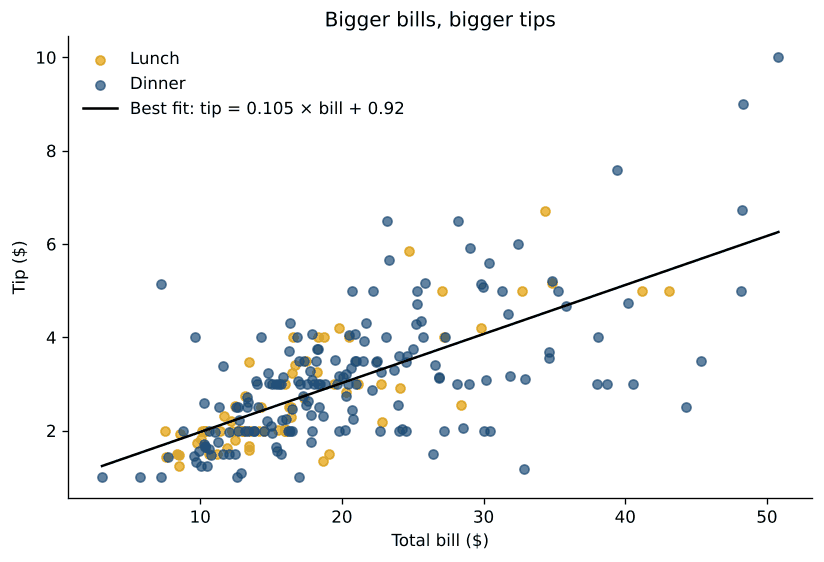
Output:
slope 0.105, intercept 0.92The slope says that, on average, each extra $10 on the bill adds about $1.05 to the tip, roughly the 10 to 20% you’d expect. The spread around the line grows with the bill: big bills get both very large and very small tips. alpha=0.7 makes dots slightly transparent so overlapping points show up as darker areas. To measure how strong the relationship is, paste the two columns into our correlation calculator, or see linear regression explained for fitting lines properly.
Pie charts, and when to use a bar chart instead
Matplotlib draws pie charts with ax.pie(). autopct prints each slice’s percentage, and startangle=90, counterclock=False starts at 12 o’clock and goes clockwise, the way people read a clock. Here the same data is shown both ways:
counts = tips["day"].value_counts().reindex(["Thur", "Fri", "Sat", "Sun"])
colors = ["#1f4e79", "#e69f00", "#7f7f7f", "#c8242c"]

fig, (ax1, ax2) = plt.subplots(1, 2, figsize=(10, 4.2))
ax1.pie(counts, labels=counts.index, autopct="%1.0f%%", colors=colors,
        startangle=90, counterclock=False, wedgeprops=dict(edgecolor="white"))
ax1.set_title("Pie chart")

ax2.bar(counts.index, counts.values, color=colors)
ax2.bar_label(ax2.containers[0])
ax2.set_title("The same data as a bar chart")
ax2.set_ylabel("Number of bills")
ax2.spines[["top", "right"]].set_visible(False)

fig.suptitle("Bills by day")
fig.savefig("pie.png", dpi=150, bbox_inches="tight")
plt.show()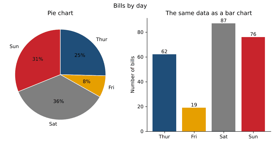
People judge lengths far more accurately than angles or areas. In the pie, Saturday and Sunday look about the same size; in the bar chart it’s obvious Saturday is bigger, and the exact counts are on the bars. Use a pie only for a few parts of one whole, ideally two or three, and use a bar chart for everything else.
Multiple plots in one figure
plt.subplots(rows, cols) returns a grid of axes you index like a table: axes[0, 0] is the top-left chart. layout="constrained" spaces them so titles and labels don’t overlap.
fig, axes = plt.subplots(2, 2, figsize=(10, 7), layout="constrained")

axes[0, 0].plot(flights.groupby("year")["passengers"].sum(), marker="o", color="#1f4e79")
axes[0, 0].set_title("Passengers per year")

axes[0, 1].hist(tips["total_bill"], bins=20, color="#1f4e79", edgecolor="white")
axes[0, 1].set_title("Total bill ($)")

sizes = sorted(tips["size"].unique())
axes[1, 0].boxplot([tips.loc[tips["size"] == n, "tip_pct"] for n in sizes], tick_labels=sizes)
axes[1, 0].set_title("Tip % by party size")
axes[1, 0].set_xlabel("People at the table")

axes[1, 1].scatter(tips["size"], tips["tip"], alpha=0.4, color="#1f4e79")
axes[1, 1].set_title("Tip ($) by party size")

for ax in axes.flat:
    ax.spines[["top", "right"]].set_visible(False)

fig.suptitle("Restaurant tips at a glance", fontsize=14)
fig.savefig("grid.png", dpi=150)
plt.show()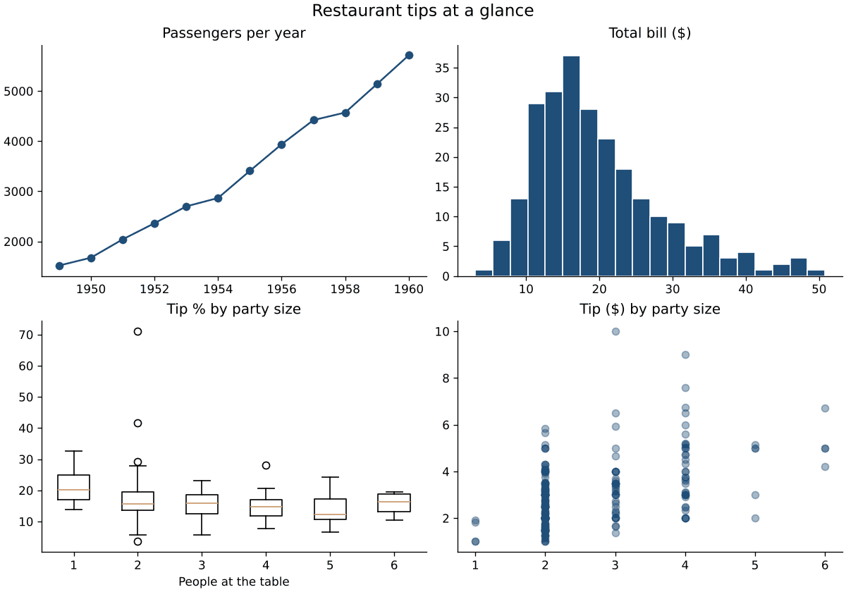
Add sharex=True or sharey=True to plt.subplots() when charts show the same variable, so they use the same scale and can be compared directly. The box plot uses tick_labels, which needs Matplotlib 3.9 or later; on older versions the argument is called labels. axes.flat loops over every chart in the grid, handy for styling them all at once.
Plot a point, add lines and shade a region
These small additions answer a lot of “how do I…” questions:
fig, ax = plt.subplots(figsize=(6, 4))
ax.plot([1, 2, 3, 4], [2, 4, 3, 5], color="lightgray")
ax.plot(3, 3, "o", color="#c8242c", markersize=10)        # a single point
ax.annotate("this point", xy=(3, 3), xytext=(3.2, 2.4), arrowprops=dict(arrowstyle="->"))
ax.axhline(4, color="gray", linestyle=":")                   # horizontal line at y=4
ax.axvline(2, color="gray", linestyle=":")                   # vertical line at x=2
ax.axvspan(3.5, 4, color="#1f4e79", alpha=0.1)               # shaded band
plt.show()
ax.axhline() and ax.axvline() draw lines across the whole chart, which is useful for targets, averages and dates. ax.axvspan() and ax.axhspan() shade a range, such as a recession or a test period. The format string "o" in ax.plot(3, 3, "o") means “draw a marker, not a line”, so a single point appears.
Which chart should you use?
| You want to show | Use | Matplotlib method |
|---|---|---|
| Change over time | Line chart | ax.plot() |
| A comparison between categories | Bar chart, sorted | ax.bar(), ax.barh() |
| The distribution of one variable | Histogram or box plot | ax.hist(), ax.boxplot() |
| The relationship between two variables | Scatter plot | ax.scatter() |
| Parts of a whole (2 or 3 parts) | Pie chart or stacked bar | ax.pie(), ax.bar(bottom=...) |
| Values across two categories | Heatmap | ax.imshow(), ax.pcolormesh() |
Make your charts look professional
- Make the title the finding. “Bigger bills, bigger tips” tells the reader what to see; “Tip vs total bill” makes them work it out.
- Label axes with units, such as “Total bill ($)” or “Passengers (thousands)”.
- Remove what doesn’t carry information: the top and right borders, unnecessary gridlines, legends for a single series.
- Use colour on purpose. One colour for everything, plus a highlight colour for what matters. The orange and dark blue used above stay distinguishable for people with the most common types of colour blindness, unlike red and green.
- Set sizes once.
plt.rcParams["font.size"] = 12at the top of a notebook changes text size for every chart, andplt.style.use("seaborn-v0_8-whitegrid")or"ggplot"applies a ready-made style.plt.style.availablelists them all.
Save charts as image files
fig.savefig("chart.png", dpi=200, bbox_inches="tight")   # for documents and slides
fig.savefig("chart.svg", bbox_inches="tight")            # sharp at any size, for the web
fig.savefig("chart.pdf", bbox_inches="tight") # for print and LaTeX- PNG works everywhere.
dpi=200gives sharp results in documents and slides; the default of 100 can look blurry. - SVG and PDF are vector formats that stay sharp at any size, ideal for web pages, print and papers.
bbox_inches="tight"trims extra white space and stops long labels from being cut off.- Save before calling
plt.show(). If you useplt.savefig()after it, the figure has usually been closed and you get a blank image;fig.savefig()on the figure object avoids the problem.
Common problems and how to fix them
| Problem | Fix |
|---|---|
| The chart doesn’t appear when running a script | Add plt.show() at the end. In Jupyter, make sure the figure is created in the cell you run. |
| The saved image is blank | Save before plt.show(), and use fig.savefig() rather than plt.savefig(). |
| Titles and labels overlap between subplots | Use plt.subplots(..., layout="constrained"). |
| Date labels on the x-axis are crowded or overlap | Call fig.autofmt_xdate() to rotate them, or convert the column with pd.to_datetime() so Matplotlib picks sensible ticks. |
| Warning: “More than 20 figures have been opened” | Close figures you’ve finished with: plt.close(fig), or plt.close("all") in loops. |
| Long category labels are cut off | Use a horizontal bar chart and bbox_inches="tight" when saving. |
TypeError about tick_labels in boxplot() | You’re on Matplotlib older than 3.9: use labels= or upgrade with pip install -U matplotlib. |
Matplotlib, seaborn or Plotly?
- Matplotlib gives full control and works everywhere, from notebooks to scripts to servers. It’s the best choice for publication-quality static charts and anything custom.
- seaborn is built on Matplotlib and makes statistical charts (distributions, regression lines, heatmaps, charts split by category) in one line each, with good defaults. Because it returns Matplotlib axes, everything in this guide still works on seaborn charts.
- Plotly makes interactive charts with zoom and hover tooltips, which is best for dashboards and web pages. See our Plotly tutorial.
Many analysts use seaborn or pandas’ .plot() for quick exploration and Matplotlib to polish the final chart. Our exploratory data analysis tutorial shows charts in the context of a full analysis.
Related tutorials
- Exploratory data analysis in Python
- Interactive visualizations with Plotly
- Data manipulation with pandas
- How to build a data dashboard
- Free descriptive statistics calculator
The official Matplotlib documentation has a gallery of examples and the full reference for every function used here.
FAQ
What is Matplotlib used for?
Creating charts in Python: line charts, bar charts, histograms, scatter plots, maps, heatmaps and almost any custom figure. It’s used in data analysis, science and engineering, and it’s the foundation for pandas plotting and seaborn.
Is Matplotlib hard to learn?
The basics take an hour: create fig, ax, call a plotting method, add labels. The large API can feel overwhelming, but most charts need the same dozen methods shown in this guide. Look up the rest when you need it.
Should I learn Matplotlib or seaborn first?
Learn the Matplotlib basics first, because seaborn charts are Matplotlib charts underneath. Once you know fig and ax, you can customize any seaborn chart with the same methods.
How do I change the size of a chart?
Pass figsize=(width, height) in inches to plt.subplots(), for example plt.subplots(figsize=(10, 5)). For sharper saved images, raise dpi in savefig() rather than the figure size.
How do I draw a line of best fit in Matplotlib?
Fit it with NumPy, slope, intercept = np.polyfit(x, y, 1), then plot slope * x + intercept with ax.plot(), as in the scatter plot example above.
How do I plot multiple lines on one chart?
Call ax.plot() once per line on the same axes, give each a label=, and finish with ax.legend().
