
Principal component analysis (PCA) takes a dataset with many columns and finds a smaller set of new columns that keep most of the information. It’s used to visualize high-dimensional data, speed up models and remove redundancy between features.
This guide explains how PCA works in plain terms, then walks through it in Python with scikit-learn on two built-in datasets. Every output shown is what the code printed when we ran it.
PCA in one paragraph
Imagine a cloud of points. PCA finds the direction in which the points are most spread out and calls it the first principal component (PC1). It then finds the next most spread-out direction that is at right angles to the first (PC2), and so on. Each component is a weighted mix of the original columns. Because the first few components capture most of the spread, or variance, you can often keep just those and drop the rest with little loss.
Three terms you’ll see throughout:
- Explained variance ratio: the share of the total variance each component captures.
- Loadings: the weights that say how much each original column contributes to a component.
- Scores: each row’s coordinates on the new components, i.e. the transformed data.
Step 1: Load the data
pip install scikit-learn pandas matplotlibThe wine dataset has 13 chemical measurements for 178 wines from three cultivars (grape varieties) grown in the same region of Italy.
from sklearn.datasets import load_wine
import pandas as pd

wine = load_wine(as_frame=True)
X, y = wine.data, wine.target

print(X.shape)
print(y.value_counts().sort_index().to_dict())
print(X.describe().loc[["mean", "std"], ["alcohol", "magnesium", "proline"]].round(2))
Output:
(178, 13)
{0: 59, 1: 71, 2: 48}
      alcohol  magnesium  proline
mean    13.00      99.74   746.89
std      0.81      14.28   314.91
Look at the scales. Alcohol varies by less than 1 unit, while proline varies by more than 300. That difference matters a lot for PCA.
Step 2: Always scale first
Here’s what happens if you run PCA on the raw data:
from sklearn.decomposition import PCA

pca_raw = PCA().fit(X)
print(pca_raw.explained_variance_ratio_[:3].round(3))
print(X.columns[abs(pca_raw.components_[0]).argmax()])
Output:
[0.998 0.002 0.   ]
proline
The first component claims 99.8% of the variance, and it’s almost entirely proline. That isn’t an insight about wine. Proline is simply measured in much bigger numbers, so it dominates any calculation based on variance.
Standardize the columns first so each has a mean of 0 and a standard deviation of 1, then fit PCA again:
from sklearn.preprocessing import StandardScaler

X_scaled = StandardScaler().fit_transform(X)
pca = PCA().fit(X_scaled)

print(pca.explained_variance_ratio_.round(3))
print(pca.explained_variance_ratio_.cumsum().round(3))
Output:
[0.362 0.192 0.111 0.071 0.066 0.049 0.042 0.027 0.022 0.019 0.017 0.013
 0.008]
[0.362 0.554 0.665 0.736 0.802 0.851 0.893 0.92  0.942 0.962 0.979 0.992
 1.   ]
Now the variance is shared sensibly. PC1 captures 36.2%, PC2 another 19.2%, and together the first two hold 55.4% of the information in all 13 columns.
Step 3: Decide how many components to keep
There’s no single right number. A common approach is to keep enough components to explain a target share of the variance, often 80% to 95%.
import numpy as np

cumulative = pca.explained_variance_ratio_.cumsum()
print(np.argmax(cumulative >= 0.80) + 1)
print(np.argmax(cumulative >= 0.95) + 1)

# Or let scikit-learn choose: keep enough components for 95% of the variance
print(PCA(n_components=0.95).fit(X_scaled).n_components_)
Output:
5
10
10
Five components reach 80% and ten reach 95%. Passing a number between 0 and 1 as n_components lets scikit-learn pick the count for you. A cumulative variance plot shows the same thing visually:
import matplotlib.pyplot as plt

fig, ax = plt.subplots(figsize=(7, 4))
ax.plot(range(1, 14), cumulative, marker="o")
ax.axhline(0.95, linestyle="--", color="grey")
ax.set_xlabel("Number of components")
ax.set_ylabel("Cumulative explained variance")
plt.show()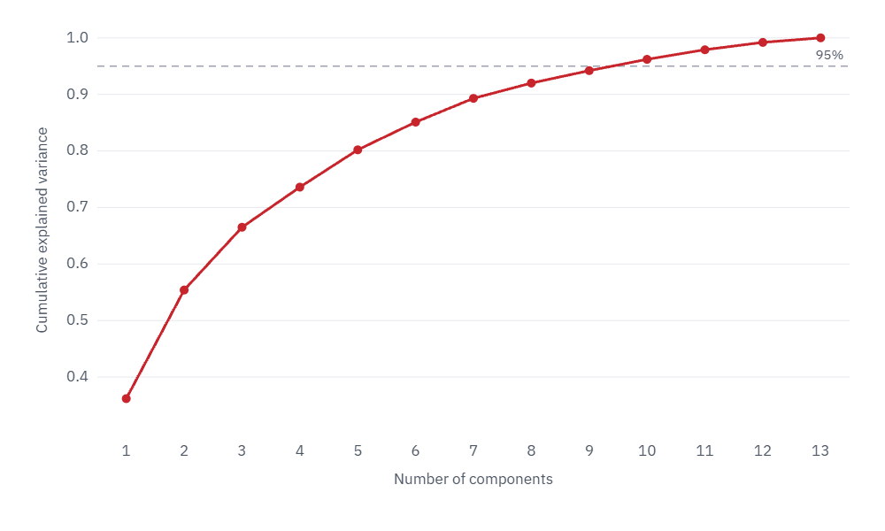
If the goal is a chart, you keep two. If the goal is a smaller input for a model, test a few values, as in Step 6.
Step 4: Project the data and plot it
pca2 = PCA(n_components=2)
X_2d = pca2.fit_transform(X_scaled)

print(X_2d.shape)
print(X_2d[:3].round(2))
Output:
(178, 2)
[[ 3.32  1.44]
 [ 2.21 -0.33]
 [ 2.52  1.03]]
Each wine is now described by two numbers instead of 13. Plot them, coloring each point by cultivar:
import matplotlib.pyplot as plt

fig, ax = plt.subplots(figsize=(7, 5))
for cls, name in enumerate(wine.target_names):
    points = X_2d[y == cls]
    ax.scatter(points[:, 0], points[:, 1], label=name, alpha=0.8)
ax.set_xlabel(f"PC1 ({pca2.explained_variance_ratio_[0]:.0%} of variance)")
ax.set_ylabel(f"PC2 ({pca2.explained_variance_ratio_[1]:.0%} of variance)")
ax.legend()
plt.show()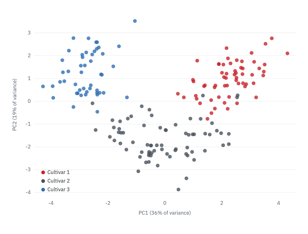
PCA is unsupervised: it never saw which cultivar each wine belongs to. The fact that the three groups still separate so clearly tells you the chemical differences between cultivars are the biggest source of variation in this data.
Step 5: Interpret the components
A component is only useful if you can say what it means. The loadings show which original columns drive each one:
loadings = pd.DataFrame(pca2.components_.T, index=X.columns, columns=["PC1", "PC2"])
print(loadings.reindex(loadings["PC1"].abs().sort_values(ascending=False).index).head(5).round(2))
print(loadings.reindex(loadings["PC2"].abs().sort_values(ascending=False).index).head(5).round(2))
Output:
                               PC1   PC2
flavanoids                    0.42 -0.00
total_phenols                 0.39  0.07
od280/od315_of_diluted_wines  0.38 -0.16
proanthocyanins               0.31  0.04
nonflavanoid_phenols         -0.30  0.03
                  PC1   PC2
color_intensity -0.09  0.53
alcohol          0.14  0.48
proline          0.29  0.36
ash             -0.00  0.32
magnesium 0.14 0.30- PC1 is mostly about phenolic compounds: flavanoids, total phenols and related measures all load positively, and nonflavanoid phenols load negatively. Wines on the right of the plot are rich in phenols.
- PC2 is mostly about color intensity and alcohol. Wines near the top are darker and stronger.
You may get the same numbers with the signs flipped. That’s normal; the direction of a component is arbitrary, and flipping it doesn’t change the result.
Step 6: Use PCA before a model
PCA is often used to shrink the input to a model. The test that matters is whether accuracy holds up. Put scaling, PCA and the model in one pipeline, so each cross-validation fold learns the scaling and components from its own training data only:
from sklearn.pipeline import make_pipeline
from sklearn.linear_model import LogisticRegression
from sklearn.model_selection import cross_val_score

for k in [1, 2, 3, 5, 13]:
    pipe = make_pipeline(StandardScaler(), PCA(n_components=k), LogisticRegression(max_iter=1000))
    score = cross_val_score(pipe, X, y, cv=5).mean()
    print(k, round(score, 3))
Output:
1 0.849
2 0.955
3 0.961
5 0.978
13 0.983| Components kept | Cross-validated accuracy |
|---|---|
| 1 | 84.9% |
| 2 | 95.5% |
| 3 | 96.1% |
| 5 | 97.8% |
| 13 (all) | 98.3% |
Two components get within three points of using every feature, and five get within half a point. With 13 columns that saving doesn’t matter much. With thousands of columns, such as pixels, gene measurements or word counts, it makes models faster to train and less likely to overfit.
Step 7: A bigger example, compressing images
The digits dataset contains 1,797 handwritten digits, each an 8×8 image stored as 64 pixel values.
from sklearn.datasets import load_digits

digits = load_digits()
print(digits.data.shape)

pca_d = PCA(n_components=0.95).fit(digits.data)
print(pca_d.n_components_)
Output:
(1797, 64)
29
Twenty-nine components keep 95% of the variance, less than half the original 64 values. To see what you lose, compress the images and turn them back into pixels with inverse_transform:
for k in [5, 10, 20, 29]:
    p = PCA(n_components=k).fit(digits.data)
    restored = p.inverse_transform(p.transform(digits.data))
    error = ((digits.data - restored) ** 2).mean()
    print(k, round(p.explained_variance_ratio_.sum(), 3), round(error, 2))
Output:
5 0.545 8.54
10 0.738 4.91
20 0.894 1.98
29 0.955 0.85
The columns are components kept, variance explained and average reconstruction error. The pixels don’t need scaling here because they all share the same 0 to 16 scale.
fig, axes = plt.subplots(4, 6, figsize=(7, 5))
for row, k in enumerate([None, 5, 10, 29]):
    if k is None:
        images = digits.data
    else:
        p = PCA(n_components=k).fit(digits.data)
        images = p.inverse_transform(p.transform(digits.data))
    for col in range(6):
        axes[row, col].imshow(images[col].reshape(8, 8), cmap="gray_r")
        axes[row, col].axis("off")
    axes[row, 0].set_title("original" if k is None else f"{k} components", loc="left", fontsize=9)
plt.tight_layout()
plt.show()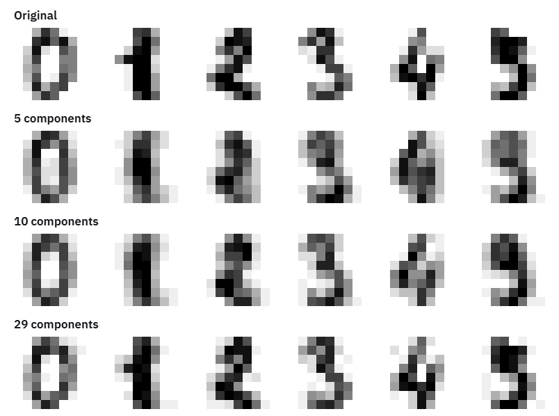
With 5 components the digits are blurry but mostly recognizable. With 29 they’re nearly indistinguishable from the originals, using less than half the data.
When not to use PCA
- When you need to explain individual features. A model built on components can’t tell you directly how alcohol affects the prediction.
- When relationships are strongly non-linear. PCA only finds straight-line directions. For visualizing complex structure, t-SNE or UMAP often show clusters PCA misses.
- When you have few columns. With 5 or 10 features, the gain is usually too small to justify the loss of interpretability.
- On unscaled data with mixed units, unless you have a specific reason, as Step 2 showed.
Common mistakes
- Forgetting to scale. The column with the biggest numbers wins, as proline did.
- Fitting PCA on all the data before splitting. Fit it inside a pipeline so test data never influences the components.
- Treating components as original features. PC1 isn’t “flavanoids”; it’s a weighted mix. Check the loadings before naming it.
- Keeping too few components for a model. Two components were great for the chart but cost three points of accuracy. Choose by testing.
Keep learning
- K-means clustering: PCA and clustering are often used together
- Logistic regression explained: the model used in Step 6
- How to clean and preprocess data using Python
- Exploratory data analysis in Python
The scikit-learn user guide on PCA covers the PCA class and its variants in more detail.
FAQ
What does PCA do, in simple terms?
It finds the few directions in your data where the values vary the most, and lets you describe each row using those directions instead of all the original columns.
Do I need to scale data before PCA?
Almost always, yes, when columns are in different units. Without scaling, the column with the largest numbers dominates the result. On the wine data, unscaled PCA put 99.8% of the variance on one column.
How many principal components should I keep?
Keep enough to explain a target share of the variance, often 80% to 95%, or test several values and keep the smallest number that doesn’t hurt your model. Use two or three for visualization.
Is PCA supervised or unsupervised?
Unsupervised. It never uses the target labels. That’s why it can show natural groupings, but also why the components it finds aren’t guaranteed to be the most useful ones for prediction.
What’s the difference between PCA and feature selection?
Feature selection keeps some of the original columns and drops others. PCA creates new columns that are mixtures of all the originals. Feature selection is easier to interpret; PCA usually keeps more information in fewer columns.
